A Basic Introduction to
Feedforward Backpropagation Neural Networks
(after Leverington, 2001)
|
The Feedforward Backpropagation Neural Network Algorithm
Although the long-term goal of the neural-network community remains the design of autonomous machine intelligence, the main modern application of artificial neural networks is in the field of pattern recognition (e.g., Joshi et al., 1997). In the sub-field of data classification, neural-network methods have been found to be useful alternatives to statistical techniques such as those which involve regression analysis or probability density estimation (e.g., Holmström et al., 1997). The potential utility of neural networks in the classification of multisource satellite-imagery databases has been recognized for well over a decade, and today neural networks are an established tool in the field of remote sensing.
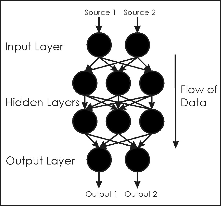
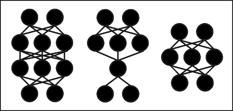
Neural networks are members of a family of computational architectures inspired by biological brains (e.g., McClelland et al., 1986; Luger and Stubblefield, 1993). Such architectures are commonly called "connectionist systems", and are composed of interconnected and interacting components called nodes or neurons (these terms are generally considered synonyms in connectionist terminology, and are used interchangeably here). Neural networks are characterized by a lack of explicit representation of knowledge; there are no symbols or values that directly correspond to classes of interest. Rather, knowledge is implicitly represented in the patterns of interactions between network components (Lugar and Stubblefield, 1993). A graphical depiction of a typical feedforward neural network is given in Figure 1. The term “feedforward” indicates that the network has links that extend in only one direction. Except during training, there are no backward links in a feedforward network; all links proceed from input nodes toward output nodes.
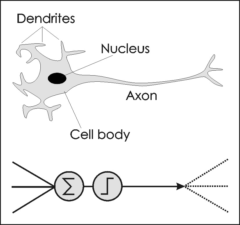
Individual nodes in a neural network emulate biological neurons by taking input data and performing simple operations on the data, selectively passing the results on to other neurons (Figure 2). The output of each node is called its "activation" (the terms "node values" and "activations" are used interchangeably here). Weight values are associated with each vector and node in the network, and these values constrain how input data (e.g., satellite image values) are related to output data (e.g., land-cover classes). Weight values associated with individual nodes are also known as biases. Weight values are determined by the iterative flow of training data through the network (i.e., weight values are established during a training phase in which the network learns how to identify particular classes by their typical input data characteristics). A more formal description of the foundations of multi-layer, feedforward, backpropagation neural networks is given in Section 5.
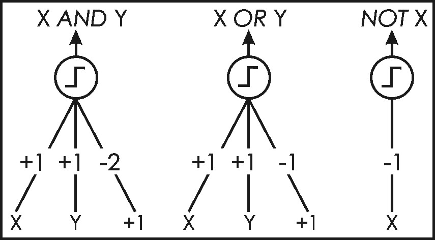
Neural computing began with the development of the McCulloch-Pitts network in the 1940's (McCulloch and Pitts, 1943; Luger and Stubblefield, 1993). These simple connectionist networks, shown in Figure 3, are stand-alone “decision machines” that take a set of inputs, multiply these inputs by associated weights, and output a value based on the sum of these products. Input values (also known as input activations) are thus related to output values (output activations) by simple mathematical operations involving weights associated with network links. McCulloch-Pitts networks are strictly binary; they take as input and produce as output only 0's or 1's. These 0's and 1's can be thought of as excitatory or inhibitory entities, respectively (Luger and Stubblefield, 1993). If the sum of the products of the inputs and their respective weights is greater than or equal to 0, the output node returns a 1 (otherwise, a 0 is returned). The value of 0 is thus a threshold that must be exceeded or equalled if the output of the system is to be 1. The above rule, which governs the manner in which an output node maps input values to output values, is known as an activation function (meaning that this function is used to determine the activation of the output node). McCulloch-Pitts networks can be constructed to compute logical functions (for example, in the “X AND Y” case, no combination of inputs can produce a sum of products that is greater than or equal to 0, except the combination X=Y=1). McCulloch-Pitts networks do not learn, and thus the weight values must be determined in advance using other mathematical or heuristic means. Nevertheless, these networks did much to inspire further research into connectionist models during the 1950's (Luger and Stubblefield, 1993).
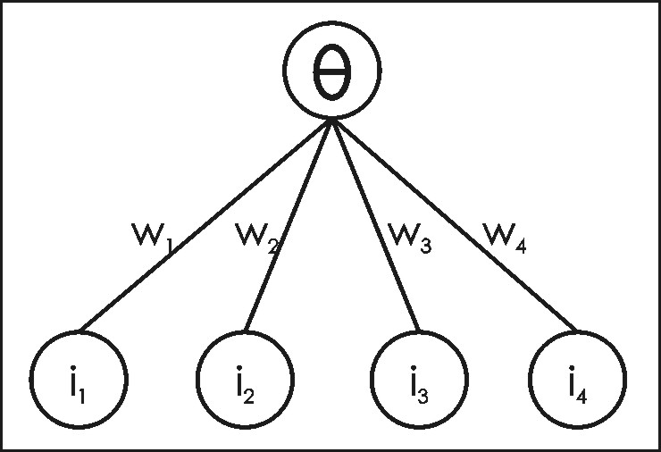
The development of a connectionist system capable of limited learning occurred in the late 1950's, when Rosenblatt created a system known as a perceptron (see Rosenblatt, 1962; Luger and Stubblefield, 1993). Again, this system consists of binary activations (inputs and outputs) (see Figure 4). In common with the McCulloch-Pitts neuron described above, the perceptron’s binary output is determined by summing the products of inputs and their respective weight values. In the perceptron implementation, a variable threshold value is used (whereas in the McCulloch-Pitts network, this threshold is fixed at 0): if the linear sum of the input/weight products is greater than a threshold value (theta), the output of the system is 1 (otherwise, a 0 is returned). The output unit is thus said to be, like the perceptron output unit, a linear threshold unit. To summarize, the perceptron “classifies” input values as either 1 or 0, according to the following rule, referred to as the activation function:
(eqn 1) The perceptron is trained (i.e., the weights and threshold values are calculated) based on an iterative training phase involving training data. Training data are composed of a list of input values and their associated desired output values. In the training phase, the inputs and related outputs of the training data are repeatedly submitted to the perceptron. The perceptron calculates an output value for each set of input values. If the output of a particular training case is labelled 1 when it should be labelled 0, the threshold value (theta) is increased by 1, and all weight values associated with inputs of 1 are decreased by 1. The opposite is performed if the output of a training case is labelled 0 when it should be labelled 1. No changes are made to the threshold value or weights if a particular training case is correctly classified. This set of training rules is summarized as:
(eqn 2a) where the subscript x refers to a particular input-node and weight pair. The effect of the above training rules is to make it less likely that a particular error will be made in subsequent training iterations. For example, in equation (2b), increasing the threshold value serves to make it less likely that the same sum of products will exceed the threshold in later training iterations, and thus makes it less likely that an output value of 1 will be produced when the same inputs are presented. Also, by modifying only those weights that are associated with input values of 1, only those weights that could have contributed to the error are changed (weights associated with input values of 0 are not considered to have contributed to error). Once the network is trained, it can be used to classify new data sets whose input/output associations are similar to those that characterize the training data set. Thus, through an iterative training stage in which the weights and threshold gradually migrate to useful values (i.e., values that minimize or eliminate error), the perceptron can be said to “learn” how to solve simple problems.
Figure 4: An example of a perceptron. The system consists of binary activations. Weights are identified by w’s, and inputs are identified by i’s. A variable threshold value (theta) is used at the output node. The development of the perceptron was a large step toward the goal of creating useful connectionist networks capable of learning complex relations between inputs and outputs. In the late 1950's, the connectionist community understood that what was needed for the further development of connectionist models was a mathematically-derived (and thus potentially more flexible and powerful) rule for learning. By the early 1960's, the Delta Rule [also known as the Widrow and Hoff learning rule or the least mean square (LMS) rule] was invented (Widrow and Hoff, 1960). This rule is similar to the perceptron learning rule above (McClelland and Rumelhart, 1988), but is also characterized by a mathematical utility and elegance missing in the perceptron and other early learning rules. The Delta Rule uses the difference between target activation (i.e., target output values) and obtained activation to drive learning. For reasons discussed below, the use of a threshold activation function (as used in both the McCulloch-Pitts network and the perceptron) is dropped; instead, a linear sum of products is used to calculate the activation of the output neuron (alternative activation functions can also be applied - see Section 5.2). Thus, the activation function in this case is called a linear activation function, in which the output node’s activation is simply equal to the sum of the network’s respective input/weight products. The strengths of network’s connections (i.e., the values of the weights) are adjusted to reduce the difference between target and actual output activation (i.e., error). A graphical depiction of a simple two-layer network capable of employing the Delta Rule is given in Figure 5. Note that such a network is not limited to having only one output node.
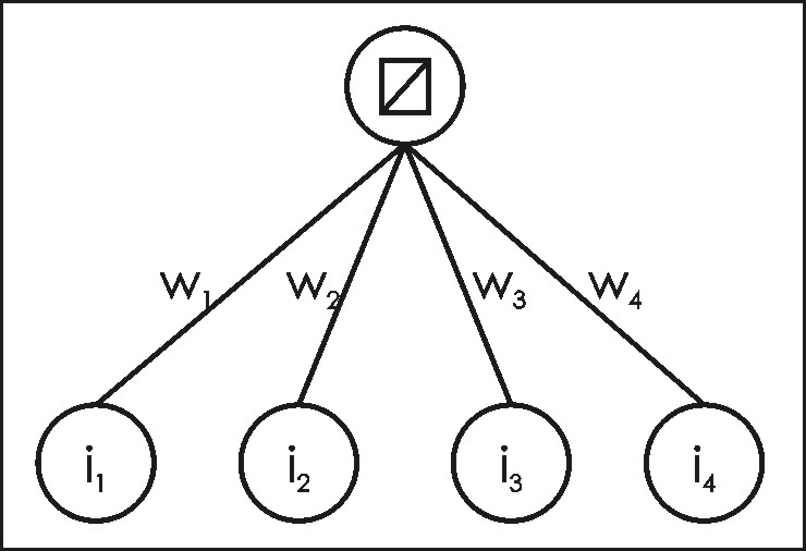
Figure 5: A network capable of implementing the Delta Rule. Non-binary values may be used. Weights are identified by w’s, and inputs are identified by i’s. A simple linear sum of products (represented by the symbol at top) is used as the activation function at the output node of the network shown here. During forward propagation through a network, the output (activation) of a given node is a function of its inputs. The inputs to a node, which are simply the products of the output of preceding nodes with their associated weights, are summed and then passed through an activation function before being sent out from the node. Thus, we have the following:
(Eqn 3a) and
(Eqn 3b) where Sj is the sum of all relevant products of weights and outputs from the previous layer i, wij represents the relevant weights connecting layer i with layer j, ai represents the activations of the nodes in the previous layer i, aj is the activation of the node at hand, and f is the activation function.
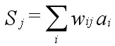
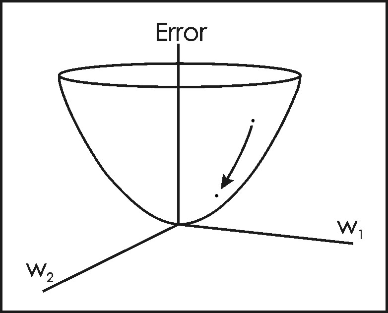
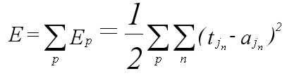
Figure 6: Schematic representation of an error function for a network containing only two weights (w1 and w2) (after Lugar and Stubblefield, 1993). Any given combination of weights will be associated with a particular error measure. The Delta Rule uses gradient descent learning to iteratively change network weights to minimize error (i.e., to locate the global minimum in the error surface). For any given set of input data and weights, there will be an associated magnitude of error, which is measured by an error function (also known as a cost function) (Figure 6) (e.g., Oh, 1997; Yam and Chow, 1997). The Delta Rule employs the error function for what is known as gradient descent learning, which involves the modification of weights along the most direct path in weight-space to minimize error; change applied to a given weight is proportional to the negative of the derivative of the error with respect to that weight (McClelland and Rumelhart 1988, pp.126-130). The error function is commonly given as the sum of the squares of the differences between all target and actual node activations for the output layer. For a particular training pattern (i.e., training case), error is thus given by:
(Eqn 4a) where Ep is total error over the training pattern, ˝ is a value applied to simplify the function’s derivative, n represents all output nodes for a given training pattern, tj sub n represents the target value for node n in output layer j, and aj sub n represents the actual activation for the same node. This particular error measure is attractive because its derivative, whose value is needed in the employment of the Delta Rule, is easily calculated. Error over an entire set of training patterns (i.e., over one iteration, or epoch) is calculated by summing all Ep:
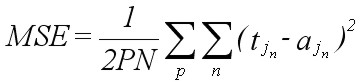
(Eqn 4b) where E is total error, and p represents all training patterns. An equivalent term for E in Equation 4b is sum-of-squares error. A normalized version of Equation 4b is given by the mean squared error (MSE) equation:
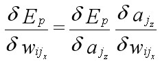
(Eqn 4c) where P and N are the total number of training patterns and output nodes, respectively. It is the error of Equations 4b and 4c that gradient descent attempts to minimize (in fact, this is not strictly true if weights are changed after each input pattern is submitted to the network; see Section 4.1 below; see also Rumelhart et al., 1986: v1, p.324; Reed and Marks, 1999: pp. 57-62). Error over a given training pattern is commonly expressed in terms of the total sum of squares (“tss”) error, which is simply equal to the sum of all squared errors over all output nodes and all training patterns. The negative of the derivative of the error function is required in order to perform gradient descent learning. The derivative of Equation 4a (which measures error for a given pattern p), with respect to a particular weight wij sub x, is given by the chain rule as:
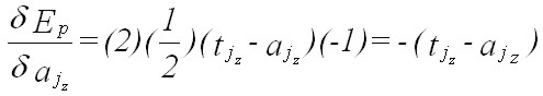
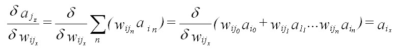
(Eqn 5a) where aj sub z is the activation of the node in the output layer that corresponds to the weight wij sub x (note: subscripts refer to particular layers of nodes or weights, and the “sub-subscripts” simply refer to individual weights and nodes within these layers). It follows that
(Eqn 5b) and
(Eqn 5c) Thus, the derivative of the error over an individual training pattern is given by the product of the derivatives of Equation 5a:
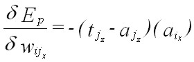
(Eqn 5d) Because gradient descent learning requires that any change in a particular weight be proportional to the negative of the derivative of the error, the change in a given weight must be proportional to the negative of equation 5d. Replacing the difference between the target and actual activation of the relevant output node by d, and introducing a learning rate epsilon, Equation 5d can be re-written in the final form of the delta rule:
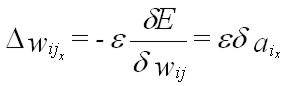
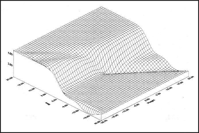
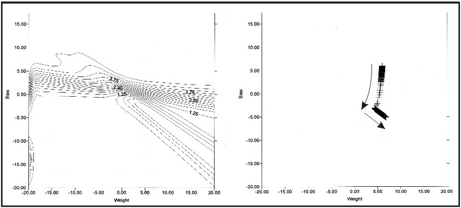
(Eqn 5e) The reasoning behind the use of a linear activation function here instead of a threshold activation function can now be justified: the threshold activation function that characterizes both the McColloch and Pitts network and the perceptron is not differentiable at the transition between the activations of 0 and 1 (slope = infinity), and its derivative is 0 over the remainder of the function. As such, the threshold activation function cannot be used in gradient descent learning. In contrast, a linear activation function (or any other function that is differentiable) allows the derivative of the error to be calculated. Equation 5e is the Delta Rule in its simplest form (McClelland and Rumelhart, 1988). From Equation 5e it can be seen that the change in any particular weight is equal to the products of 1) the learning rate epsilon, 2) the difference between the target and actual activation of the output node [d], and 3) the activation of the input node associated with the weight in question. A higher value for e will necessarily result in a greater magnitude of change. Because each weight update can reduce error only slightly, many iterations are required in order to satisfactorily minimize error (Reed and Marks, 1999). An actual example of the iterative change in neural network weight values as a function of an error surface is given in Figures 7 and 8. Figure 7 is a three-dimensional depiction of the error surface associated with a particular mathematical problem. Figure 8 shows the two-dimensional version of this error surface, along with the path that weight values took during training. Note that weight values changed such that the path defined by weight values followed the local gradient of the error surface.
Figure 8: Two-dimensional depiction of the error surface given in Figure 7, shown with the training path iteratively taken by weight values during training (starting at weight values [+6,+6]) (Leverington, 2001). Note that weight values changed such that the path defined by weight values followed the local gradient of the error surface.
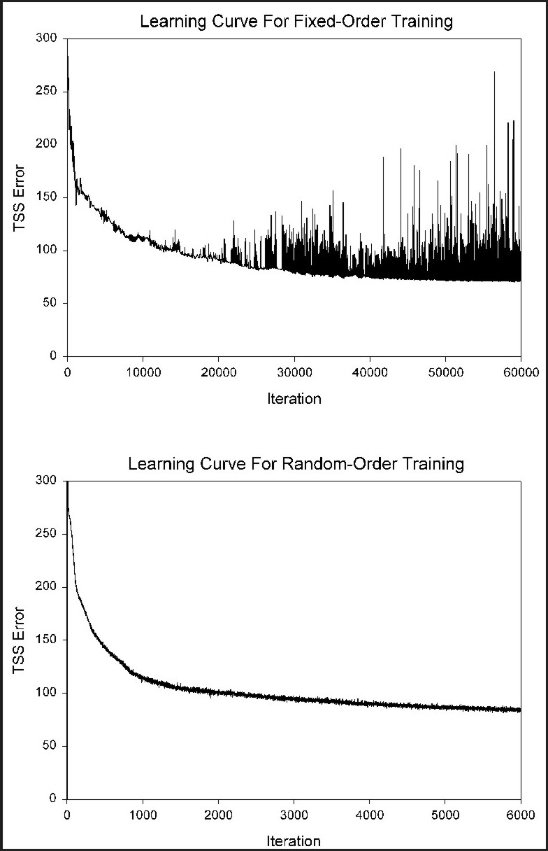
Weights can be updated in two primary ways: batch training, and on-line (also called sequential or pattern-based) training. In batch mode, the value of dEp/dwij is calculated after each pattern is submitted to the network, and the total derivative dE/dwij is calculated at the end of a given iteration by summing the individual pattern derivatives. Only after this value is calculated are the weights updated. As long as the learning rate epsilon (e) is small, batch mode approximates gradient descent (Reed and Marks, 1999). Cyclic, fixed orders of training patterns are generally avoided in on-line learning, since convergence can be limited if weights converge to a limit cycle (Reed and Marks 1999: p.61). Also, if large numbers of patterns are in a training dataset, an ordered presentation of the training cases to the network can cause weights/error to move very erratically over the error surface (with any given series of an individual class’ training patterns potentially causing the network to move in weight-space in a direction that is very different from the overall desired direction). Thus, training patterns are usually submitted at random in on-line learning. A comparison between the learning curves produced by networks using non-random and random submission of training data is given in Figure 9. Note that the network using non-random submission produced an extremely erratic learning curve, compared to the relatively smooth learning curve produced by the network using random submission. The on-line mode has an advantage over batch mode, in that the more erratic path that the weight values travel in is more likely to bounce out of local minima; pure gradient descent offers no chance to escape a local minimum. Further, the on-line mode is superior to batch mode if there is a high degree of redundancy in the training data, since, when using a large training dataset, the network will simply update weights more often in a given iteration, while a batch-mode network will simply take longer to evaluate a given iteration (Bishop, 1995a, p.264). An advantage of batch mode is that it can settle on a stable set of weight values, without wandering about this set.
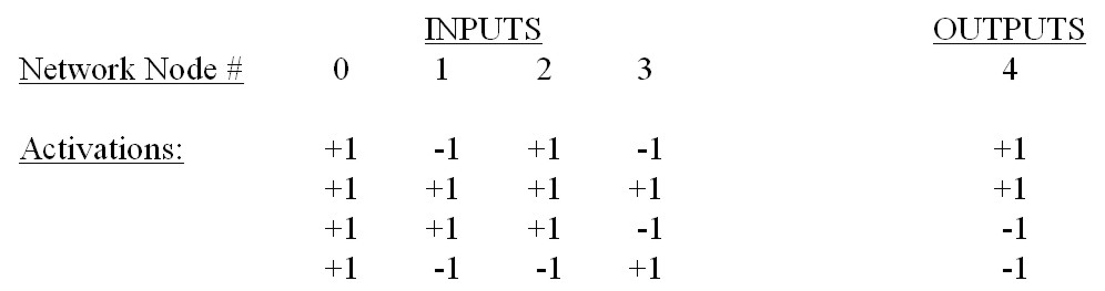
A simple example of the employment of the Delta Rule, based on a discussion given in McClelland and Rumelhart (1988), is as follows: imagine that the following inputs and outputs are related as in Table 3.1. Imagine further that is the desire of a worker is to train a network to be able to correctly label each of the four input cases in this table. This problem will require a network with four input nodes and one output node. All 4 weights associated with each input node are initially set to 0, and an arbitrary learning rate (epsilon) of 0.25 is used in this example.
After this first iteration, it is not clear that the weights are changing in a manner that will reduce network error. In fact, with the last set of weights given above, the network would only produce a correct output value for the last training case; the first three would be classified incorrectly. However, with repeated presentation of the same training data to the network (ie. with multiple iterations of training), it becomes clear that the network’s weights do indeed evolve to reduce classification error: error is eliminated altogether by the twentieth iteration. The network has learned to classify all training cases correctly, and is now ready to be used on new data whose relations between inputs and desired outputs generally match those of the training data. The Delta Rule will find a set of weights that solves a network learning problem, provided such a set of weights exists. The required condition for this set of weights existing is that all solutions must be a linear function of the inputs. As was presented by Minsky and Papert (1969), this condition does not hold for many simple problems (e.g., the exclusive-OR function, in which an output of 1 must be produced when either of two inputs are 1, but an output of 0 must be produced with neither or both of the inputs are 1; see McClelland and Rumelhart 1988, pp. 145-152). Minsky and Papert recognized that a multi-layer network could convert an “unsolvable” problem to a “solvable” problem (note: a multi-layer network consists of one or more intermediate layers placed between the input and output layers; this accepted terminology can be somewhat confusing and contradictory, in that the term “layer” in “multi-layer” refers to a row of weights, whereas the term “layer” in general neural-network usage usually means a row of nodes; see Section 5.1 and, e.g., Vemuri, 1992, p.42). Minsky and Papert also recognized that the use of a linear activation function (such as that used in the Delta Rule example above, where network output is equal to the sum of the input/weight products) would not allow the benefits of having a multi-layer network to be realized, since a multi-layer network with linear activation functions is functionally equivalent to a simple input-output network using linear activation functions. That is, linear systems cannot compute more in multiple layers than they can in a single layer (McClelland and Rumelhart, 1988). Based on the above considerations, the questions at the time became 1) what kind of activation function should be used in a multi-layer network, and 2) how can intermediate layers in a multi-layer network be “taught”? The original application of the Delta Rule involved only an input layer and an output layer. It was generally believed that no general learning rule for larger, multi-layer networks, could be formulated. As a result of this view, research on connectionist networks for applications in artificial intelligence was dramatically reduced in the 1970's (McClelland and Rumelhart, 1988; Joshi et al., 1997).
Eventually, despite the apprehensions of earlier workers, a powerful algorithm for apportioning error responsibility through a multi-layer network was formulated in the form of the backpropagation algorithm (Rumelhart et al., 1986). The backpropagation algorithm employs the Delta Rule, calculating error at output units in a manner analogous to that used in the example of Section 4.2, while error at neurons in the layer directly preceding the output layer is a function of the errors on all units that use its output. The effects of error in the output node(s) are propagated backward through the network after each training case. The essential idea of backpropagation is to combine a non-linear multi-layer perceptron-like system capable of making decisions with the objective error function of the Delta Rule (McClelland and Rumelhart, 1988).
A multi-layer, feedforward, backpropagation neural network is composed of 1) an input layer of nodes, 2) one or more intermediate (hidden) layers of nodes, and 3) an output layer of nodes (Figure 1). The output layer can consist of one or more nodes, depending on the problem at hand. In most classification applications, there will either be a single output node (the value of which will identify a predicted class), or the same number of nodes in the output layer as there are classes (under this latter scheme, the predicted class for a given set of input data will correspond to that class associated with the output node with the highest activation). As noted in Section 4.2, it is important to recognize that the term “multi-layer” is often used to refer to multiple layers of weights. This contrasts with the usual meaning of “layer”, which refers to a row of nodes (Vemuri, 1992). For clarity, it is often best to describe a particular network by its number of layers, and the number of nodes in each layer (e.g., a “4-3-5" network has an input layer with 4 nodes, a hidden layer with 3 nodes, and an output layer with 5 nodes).
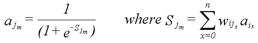
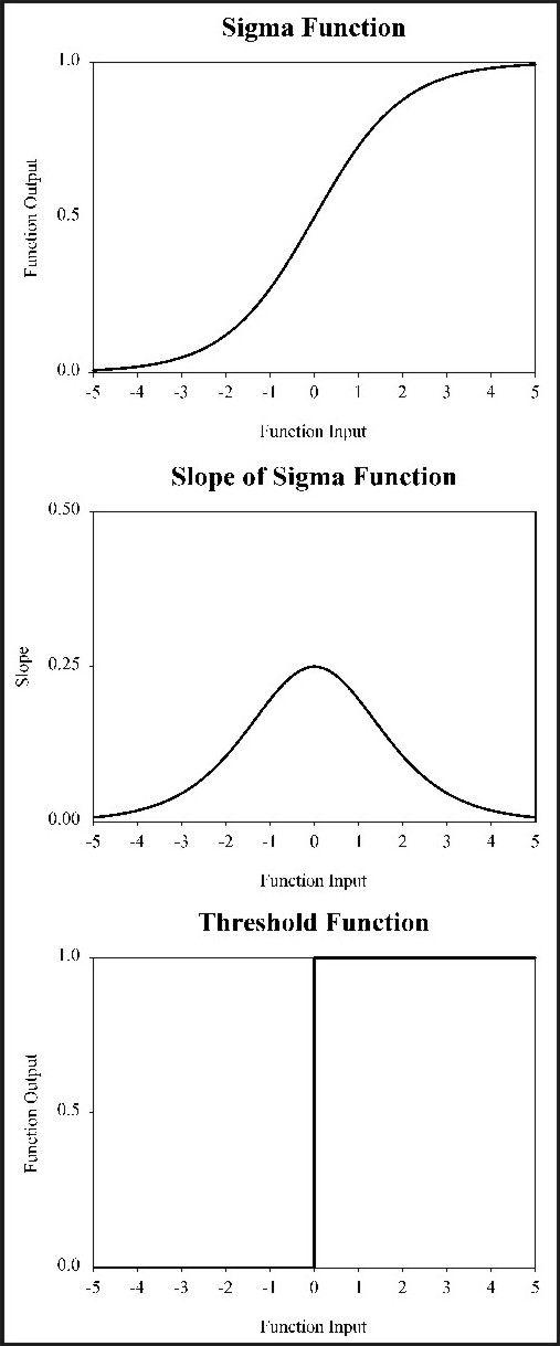
The use of a smooth, non-linear activation function is essential for use in a multi-layer network employing gradient-descent learning. An activation function commonly used in backpropagation networks is the sigma (or sigmoid) function:
(Eqn 6) where aj sub m is the activation of a particular “receiving” node m in layer j, Sj is the sum of the products of the activations of all relevant “emitting” nodes (i.e., the nodes in the preceding layer i) by their respective weights, and wij is the set of all weights between layers i and j that are associated with vectors that feed into node m of layer j. This function maps all sums into [0,1] (Figure 10) (an alternate version of the function maps activations into [-1, 1]; e.g., Gallant 1993, pp. 222-223). If the sum of the products is 0, the sigma function returns 0.5. As the sum gets larger the sigma function returns values closer to 1, while the function returns values closer to 0 as the sum gets increasingly negative. The derivative of the sigma function with respect to Sj sub m is conveniently simple, and is given by Gallant (1993, p.213) as:
(Eqn 7) The sigma function applies to all nodes in the network, except the input nodes, whose values are assigned input values. The sigma function superficially compares to the threshold function (which is used in the perceptron) as shown in Figure 10. Note that the derivative of the sigma function reaches its maximum at 0.5, and approaches its minimum with values approaching 0 or 1. Thus, the greatest change in weights will occur with values near 0.5, while the least change will occur with values near 0 or 1. McClelland and Rumelhart (1988) recognize that it is these features of the equation (i.e., the shape of the function) that contribute to the stability of learning in the network; weights are changed most for units whose values are near their midrange, and thus for those units that are not yet committed to being either “on” or “off”.
Figure 10: Graphs of the sigma function, the derivative of the sigma function, and the threshold function (after Winston, 1991; Rich and Knight, 1991).
In the employment of the backpropagation algorithm, each iteration of training involves the following steps: 1) a particular case of training data is fed through the network in a forward direction, producing results at the output layer, 2) error is calculated at the output nodes based on known target information, and the necessary changes to the weights that lead into the output layer are determined based upon this error calculation, 3) the changes to the weights that lead to the preceding network layers are determined as a function of the properties of the neurons to which they directly connect (weight changes are calculated, layer by layer, as a function of the errors determined for all subsequent layers, working backward toward the input layer) until all necessary weight changes are calculated for the entire network. The calculated weight changes are then implemented throughout the network, the next iteration begins, and the entire procedure is repeated using the next training pattern. In the case of a neural network with hidden layers, the backpropagation algorithm is given by the following three equations (modified after Gallant, 1993), where i is the “emitting” or “preceding” layer of nodes, j is the “receiving” or “subsequent” layer of nodes, k is the layer of nodes that follows j (if such a layer exists for the case at hand), ij is the layer of weights between node layers i and j, jk is the layer of weights between node layers j and k, weights are specified by w, node activations are specified by a, delta values for nodes are specified by d, subscripts refer to particular layers of nodes (i, j, k) or weights (ij, jk), “sub-subscripts” refer to individual weights and nodes in their respective layers, and epsilon is the learning rate:
(Eqn 8a)
(Eqn 8b)
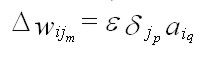
(Eqn 8c) Being based on the generalized Delta Rule, it is not surprising that Equation (8a) has the same form as Equation (5e). Equation (8a) states that the change in a given weight m located between layers i and j is equal to the products of: 1) the learning rate (epsilon); 2) the delta value for node p in layer j [where node p is the node to which the vector associated with weight m leads]; and 3) the activation of node q in layer i [where node q is the node from which the vector associated with weight m leads]. In practice, the learning rate (epsilon) is typically given a value of 0.1 or less; higher values may provide faster convergence on a solution, but may also increase instability and may lead to a failure to converge (Gallant, 1993). The delta value for node p in layer j in Equation (8a) is given either by Equation (8b) or by Equation (8c), depending on the whether or not the node is in an output or intermediate layer.
Equation (8b) gives the delta value for node p of layer j if node p is an output node. Together, Equations (8a) and (8b) were derived through exactly the same procedure as Equation 5e, with the understanding that a sigma activation function is used here instead of a simple linear activation function (use of a different activation function will typically change the value of d). Both sets of equations were determined by finding the derivative of the respective error functions with respect to any particular weight.
Equation (8c) gives the delta value for node p of layer j if node p is an intermediate node (i.e., if node p is in a hidden layer). This equation states that the delta value of a given node of interest is a function of the activation at that node (aj sub p), as well as the sum of the products of the delta values of relevant nodes in the subsequent layer with the weights associated with the vectors that connect the nodes.
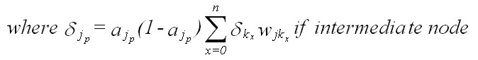
Equations (8a), (8b), and (8c) describe the main implementation of the backpropagation algorithm for multi-layer, feedforward neural networks. It should be noted, however, that most implementations of this algorithm employ an additional class of weights known as biases. Biases are values that are added to the sums calculated at each node (except input nodes) during the feedforward phase. That is, the bias associated with a particular node is added to the term Sj in Equation (3a), prior to the use of the activation function at that same node. The negative of a bias is sometimes called a threshold (Bishop, 1995a). For simplicity, biases are commonly visualized simply as values associated with each node in the intermediate and output layers of a network, but in practice are treated in exactly the same manner as other weights, with all biases simply being weights associated with vectors that lead from a single node whose location is outside of the main network and whose activation is always 1 (Figure 11). The change in a bias for a given training iteration is calculated like that for any other weight [using Equations (8a), (8b), and (8c)], with the understanding that ai sub m in Equation (8a) will always be equal to 1 for all biases in the network. The use of biases in a neural network increases the capacity of the network to solve problems by allowing the hyperplanes that separate individual classes to be offset for superior positioning. More specific discussions on the utility of biases in neural networks are given by, e.g., Gallant (1993, pp.65-66), Bishop (1995a, p.78), and Reed and Marks (1999, pp.15-17).
Figure 11: Biases are weights associated with vectors that lead from a single node whose location is outside of the main network and whose activation is always 1.
The precise network topology required to solve a particular problem usually cannot be determined (Figure 12; Castellano et al., 1997; Tamura and Tateishi, 1997; Reed and Marks, 1999; Richards and Jia, 2005), although research efforts continue in this regard. This is a critical problem in the neural-network field, since a network that is too small or too large for the problem at hand may produce poor results. This is analogous to the problem of curve fitting using polynomials: a polynomial with too few coefficients cannot evaluate a function of interest, while a polynomial with too many coefficients will fit the noise in the data and produce a poor representation of the function (e.g., Bishop, 1995a, pp.9-15; Reed and Marks, 1999, p.42).
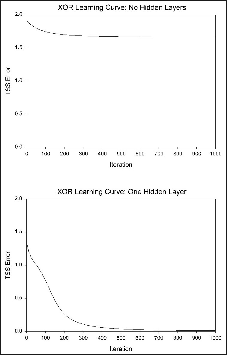
Figure 13: Learning curves for the exclusive-OR (XOR) problem (Leverington, 2001). A neural network with no hidden layers cannot solve the XOR problem (top curve), but a neural network with a single hidden layer can solve the problem with a relatively small number of iterations (bottom curve).
Although the ideal initial values for weights (i.e., those that will maximize the effectiveness and speed with which a neural network learns) cannot yet be determined theoretically (Thimm and Fiesler, 1997), it is general practice to assign randomly-generated positive and negative quantities as the initial weight values. Such a random distribution can help minimize the chances of the network becoming stuck in local minima (Gallant, 1993). Typically, values are selected from a range [-a,+a] where 0.1 < a < 2 (Reed and Marks, 1999, p.57). The reason for using random initial weights is to break symmetry, while the reason for using small initial weights is to avoid immediate saturation of the activation function (Reed and Marks, 1999, p.97). Further discussions regarding the benefits of the use of small initial weights are given by Reed and Marks (1999, p.116 and p.120).
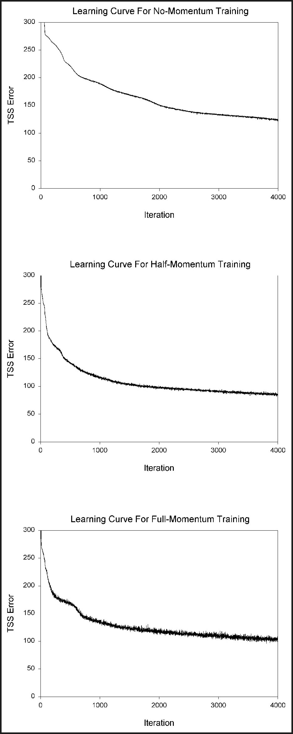
The speed of convergence of a network can be improved by increasing the learning rate epsilon. Unfortunately, increasing e will usually result in increasing network instability, with weight values oscillating erratically as they converge on a solution. Instead of changing e, most standard backpropagation algorithms employ a momentum term in order to speed convergence while avoiding instability. The momentum term is added to Equation 8a, and is equal to the product of some fraction 0 <= alpha <= 1 by the change in weight that occurred in the previous weight change. By adding fractions of previous weight changes, weight changes can be kept on a faster and more even path (Gallant, 1993).
The purpose of training a feedforward backpropagation network is to modify weight values iteratively such that the weights, over time, converge on a solution that relates inputs to outputs in a manner that is useful to the user. It is normally desirable in training for a network to be able to generalize basic relations between inputs and outputs based on training data that do not consist of all possible inputs and outputs for a given problem. A difficulty that can arise in the training of a neural network involves the adaptation of weight values so closely to training data that the utility of the network in processing new data is diminished; this problem is called over-generalization (or over-training) (e.g., Bishop, 1995a; Reed and Marks, 1999; Karystinos and Pados, 2000). In over-generalization, the network has ceased to be able to relate general ranges of values to classes, and instead relates input values to classes in a manner that is contrary to the more general relation that is desired. While early stages of learning generally result in the successful evaluation of the main features of the underlying function that properly maps inputs to outputs, later stages of learning may incorporate features of the training dataset that are uncharacteristic of the data as a whole (e.g., due to the use of incomplete or noisy training data) (Reed and Marks, 1999). Measured error in such a situation will continually be decreasing during training, but the generalization capabilities of the network will also be decreasing (as the network modifies weights to suit peculiarities of the training data being used).
One approach used to prevent over-generalization is the termination of training before over-generalization can occur (Reed and Marks, 1999). That is, for a given network, training data, and learning algorithm, there may be an optimal amount of training that produces the best generalization. While potentially effective, this solution is often not useful, since algorithms that provide information on approximately when to stop training are not necessarily dependable; such algorithms may, for example, be fooled into the premature termination of training by factors such as, e.g., local minima in the error surface. A premature halt to training will result in a network that is not trained to its highest potential, while a late halt to training can result in a network whose operation is characterized by over-generalization (Reed and Marks, 1999).
The random initialization of network weights prior to each execution of the neural network training algorithm can in some cases cause final classification results to vary from execution to execution, even when all other factors (e.g., training data, learning rate, momentum, network topology) are kept constant. Particularly when working with very limited training datasets, the variation in results can be large. Under such circumstances, it is best to expand training data on the basis of improved ground truth. If this is not possible, generation of optimum results can sometimes be made through combination of the results of multiple neural network classifications. For example, multiple neural network results can be combined using a simple consensus rule: for a given pixel, the class label with the largest number of network “votes” is that which is assigned (that is, the results of the individual neural-network executions are combined through a simple majority vote) (Hansen and Salamon, 1990). The reasoning behind such a consensus rule is that a consensus of numerous neural networks should be less fallible than any of the individual networks, with each network generating results with different error attributes as a consequence of differing weight initializations (Hansen and Salamon, 1990). Of interest in the neural network community is the use of consensus algorithms to generate final results that are superior to any individual neural network classification.
References Cited (c) David Leverington, 2009
|